In our first installment of NaviKnow’s Meteorology Month (Selecting Weather Stations for Dispersion Modeling January 10, 2018), we described a process to select an appropriate weather station to gather data from for your dispersion modeling project. In this article, we are going to walk through the process using data from the National Weather Service (NWS) and tools developed by NaviKnow. Each step will be described in detail.
The data we are using is:
- ftp://ftp.ncdc.noaa.gov/pub/data/noaa/isd-history.csv (for hourly surface observations);
- https://www1.ncdc.noaa.gov/pub/data/igra/igra2-station-list.txt (for upper air soundings); and
- http://weather.rap.ucar.edu/surface/stations.txt (for ASOS one- and five-minute data)
The files listed above do not contain the data needed to build our meteorological dataset with AERMET, but, by using NaviKnow’s Air GeoDataBase (Air GDB), you will be able to locate all available NWS stations near your project site and then, with just a click, access and download the data needed, provide the data are available from the NWS.
What is the NaviKnow Air GDB?
One of our main gripes about performing air dispersion modeling is there are dozens of places that you have to go to in order to just find the information needed (even required) to get started. When another project comes up, you have to go through the whole torturous mind numbing process all over again.
To save our own sanity, we have gone to all the sources of data that we know of and gathered ALL the data would could. We have taken ALL that data and reorganized, reformatted, and repackaged it ALL to take advantage of tools we have or have developed ourselves. So more go hinter and yon to find one little bit of obscure but necessary bit of data. It ALL lives on our desktop.
All data are in the file geodatabase format that was developed by ESRI for use with their software product ArcMap which is part of the ArcGIS suite. In order to take full advantage of the Air GDB, you would need a license of ArcMap or another GIS software product that can use the file geodatabase format.
If you do not have access to a license of ArcMap, you can still navigate through the data using a free product for ESRI called ArcReader. In ArcReader, you can access the Air GDB to look up items and perform simple tasks, but you would need ArcGIS to perform detailed queries of all the various datasets included in the Air GDB.
Let’s Get Started with the Air GDB
In this article, we will walk through the examples using ArcMap.
Remember, representativeness of the weather station(s) should be based on four criteria:
- Proximity of the NWS measurement site to the source location;
- Land use comparison between the NWS measurement site and the source location;
- Presence of large geographic features between the NWS measurement site and the source location; and
- Wind pattern and climate comparison between the NWS measurement site and the source location.
Proximity
First, launch ArcMap. To fill in your blank map, click on the Add Data icon ![]()
Locate where you have the Air GDB, then expand it to see all the datasets available. There are only two datasets to add for this example:
- WEATHER_STATIONS; and
- PROPERTY_LINES.
The PROPERTY_LINES dataset was obtained from the Texas Commission on Environmental Quality (TCEQ). It contains property boundaries of industrial sites in Texas. This dataset is being used because an application site (industrial site seeking a permit) is needed to start the whole process. You can use any dataset you like that has an application site specific to you dispersion modeling project.
Your map display should look like this:
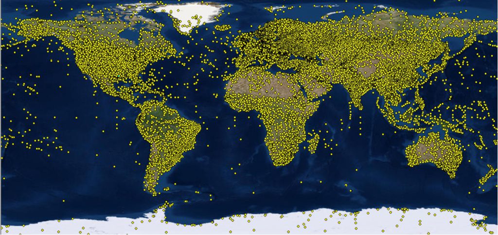
All those yellow dots (you can choose any color you like) depict the locations of weather stations that gather surface observations that are reported to the NWS/NOAA.
Next, select the location of the application site by using the Select Features icon ![]()
For this example, we have chosen a site in eastern Texas. Our map display looks like this:
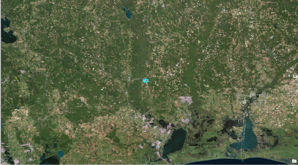
The selected site property line appears in bright blue. Your map display should be similar.
Now we are going to take advantage of the power of GIS data by performing a spatial query between the two datasets; PROPERTY_LINES and WEATHER_STATIONS. To do so, click on the Selection menu item and then click on Select By Location…
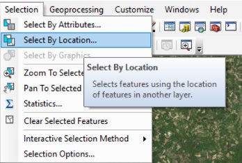
What we want to do is select features from WEATHER_STATIONS all the locations within a distance of 100 miles of the selected feature from PROPERTY_LINES. The Select By Location dialog form would look like this:
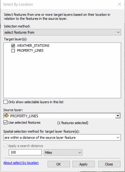
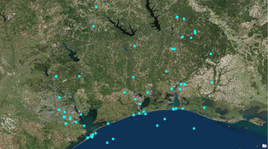
Click the Apply or OK button the execute the query. Zooming out in the map display to show all the stations meeting the query criteria (in bright blue), our display looks like this:
Selecting Appropriate Upper Air Station
The spatial query just performed selected ALL the weather stations that met our search criteria. Next we will limit the selection to just the potential upper air stations for our project.
Taking a short step back in the process, when you initially added the WEATHER_STATIONS dataset, three items, rather than one, should have appeared in the map display table of contents. The other two items are data tables that have a relationship with the data in the WEATHER_STATIONS dataset.

Since there is a relationship between the dataset and these data tables, they will automatically be accessible to you to query. This is the true power of the Air GDB. The geodatabase base allows you to drill down into the data you are looking for.
To start our query, right-click on the WEATHER_STATIONS dataset, then click on Open Attribute Table.
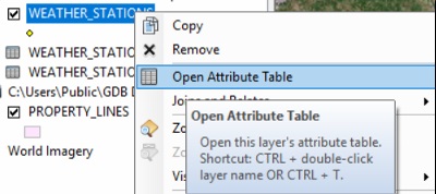
When the attribute table opens, all of the selected will appear in bright blue. We don’t need these data records, but the records from the related table WEATHER_STATIONS_UPPER_AIR. To do this, click on the related tables icon ![]()

And then select WEATHER_STATIONS_UPPER_AIR. This will open the data table containing the related records or upper air stations. You will notice that two distinct stations, Lake Charles and Shreveport, are selected. Though we see the table records, we cannot see the location of these two stations.
To see the locations of these two upper air stations, we go through the related tables in the reverse order from what we have just done. Select the related tables icon, again, but this time, select the WEATHER_STATIONS side of the relationship.

The location of the two upper air stations will be depicted in bright blue. In the map display, you can now see where the stations are located relative to the application site.
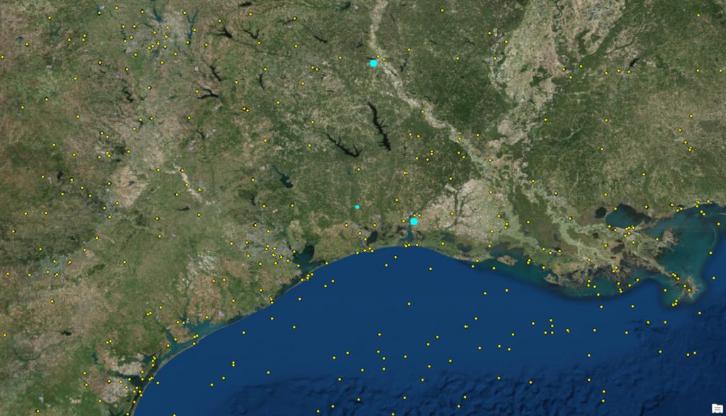
We realize this was quite a few steps for what appears to be very obvious which upper air station is closest to our application site. However, when it is not so obvious, you want to use a realistic, reproducible, systematic, and objective process that you are able to defend with minimal effort.
Land Use and Geographic Features
For the upper air stations, it is rare that the surface characteristic would significantly impact the meteorology at the upper levels of the atmosphere, however, you should do an initial comparison between the potential upper air station selections to see if there is a drastic difference. If there is a sizable difference, then make the comparison to the land use surrounding the application site.
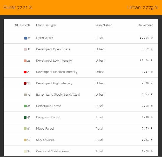
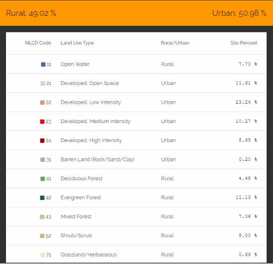
For our example, the analysis is shown below. The land use analysis was performed using NaviKnow’s Land Use Tool (http://landuse.naviknow.com/). The tool uses data from the 2011 National Land Cover Dataset (NLCD).
Lake Charles, LA
Shreveport, LA
Application Site

The land use surrounding the Lake Charles station is predominately rural, while the Shreveport station is about half and half rural to urban. Definitely a significant difference. The application site is very rural so it is more like the Lake Charles surroundings. Though proximity is the dominant factor in this case, if the stations were about equidistant from the application site, the land use analysis would be a greater factor in the final selection of which upper air station to select.
From a visual inspection of the aerial imagery and familiarity of the region, there are no significant geographic features between the stations or between the stations and the application site. The only feature that stands out is the Gulf of Mexico.
Wind pattern and Climate Comparison
The next step is to compare wind patterns between the potential upper air station selections to see if there is a drastic difference. The 30-year wind roses for the stations are below. The data were obtain from http://mrcc.isws.illinois.edu/CLIMATE/.
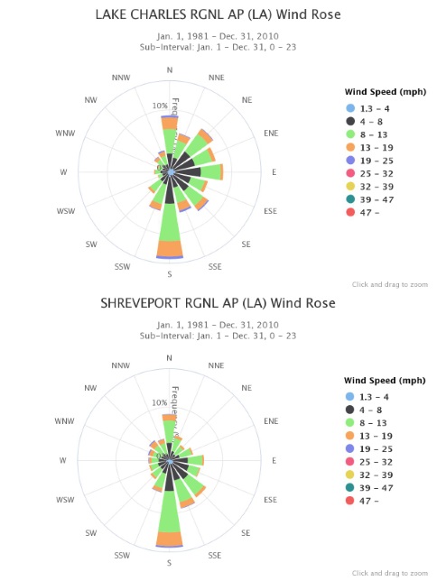
The wind patterns are similar, except for the higher percentage of winds from the east to northeast for Lake Charles. Once you get down to looking at the wind patterns of surface stations can you make a definitive selection.
Based on what we have now, our selection would be the Lake Charles station, mostly due to it being much closer (52 miles) from the application site than the Shreveport station (145 miles).
Selecting Appropriate Surface Station
The process determining an appropriate surface station are identical to that of the upper air station process with the exception of a couple of tweaks. Instead of performing a spatial query between PROPERTY_LINES and WEATHER_STATIONS using a 100 mile radius, typically you would use some less. In this example we used 50 miles, just because we saw from the first spatial query there were quite a few surface stations in the query result. Depending upon which sites have complete datasets, you may have to expand your search radius.
Proximity
As before, right-click on the WEATHER_STATIONS dataset, then click on Open Attribute Table.

Click on the related tables icon ![]()
This time, select WEATHER_STATIONS_SURFACE as shown below:

Then select the related tables icon again, then select WEATHER_STATIONS. The result will show where the locations of the surface stations that met the search criteria. In this example, it looks like this:

One note of caution: many surface stations will not have 24 hour observations so their data will not meet the 90% completeness criteria for use with AERMOD for regulatory purposes. A future enhancement is to have the completeness of dataset listed in a data field. In this example, we took the liberty of filtering out incomplete datasets. The result left two stations to choose from: the Southeast Texas Regional Airport (28 miles from the application site) and the Angelina County Airport (74 miles from the application site).
Land Use and Geographic Features
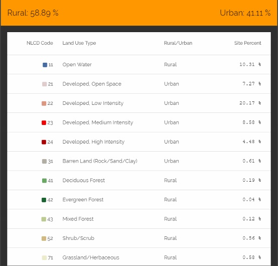
In performing the land use analysis, both potential surface stations are in surroundings that are more rural than urban. The area surrounding Southeast Texas Regional Airport is marginally more rural than urban, however, when examining the land use categories, over 20% that is considered urban is listed as land use code 22, which corresponds to residential and light commercial/retail. This does skew the percentage towards more urbanization.
Southeast Texas Regional Airport
Angelina County Airport

As before , from a visual inspection of the aerial imagery and familiarity of the region, there are no significant geographic features between to stations or between the stations and the application site. The only feature that stands out is the Gulf of Mexico.
Wind pattern and Climate Comparison
The next step is to compare wind patterns between the potential surface station selections to see if there is a drastic difference. The 30-year wind roses for the stations are below. The data were obtain from http://mrcc.isws.illinois.edu/CLIMATE/.
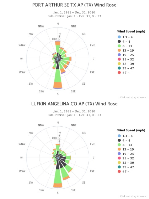
The wind patterns are similar, except for the higher percentage of winds from the east to northeast for Southeast Texas Regional Airport, similar to that of the Lake Charles station.
The Final Decision
Making the final decision as to which surface and upper air stations can be pretty straightforward or it can be very difficult. There is no easy formula. You have to use your best judgement based on the best available information.
For this example, the decision is not that difficult. Typically, proximity is the main factor and in this example, based on the information presented, proximity make the decision a lot easier. For the upper air station, Lake Charles is an easy selection since it is much closer, has similar land use, no large differences in geographic features, and similar wind patterns. For the surface station, based on the information presented, Southeast Texas Regional Airport would be my selection. It is much closer, similar (enough) land use, no large differences in geographic features, and similar wind patterns.
If you found this article informative, there is more helpful and actionable information for you. Go to http://learn.naviknow.com to see a list of past webinar mini-courses. Every Wednesday (Webinar Wednesday), NaviKnow is offering FREE webinar mini-courses on topics related to air quality dispersion modeling and air quality permitting. If you want to be on our email list, drop me a line at ceo@naviknow.com.
One of the goals of NaviKnow is to create an air quality professional community to share ideas and helpful hints like those covered in this article. So if you found this article helpful, please share with a colleague.
If you do not have the time or the tools to create meteorological input files for your AERMOD dispersion modeling project, NaviKnow is now providing a service to do it for you. If your project is in the continental US, we can do all the processing and documentation for you. Our price is 600 USD for a five-year data set. The deliverables to you are not just the files for use with AERMOD but all the inputs and outputs for AERMET Stages 1, 2, and 3, AERMINUTE, and AERSURFACE and associated documentation required by most regulatory agencies. Also, the surface characteristics will be generated using the latest land use data.
If you are interested in our meteorological data processing services, please let us know by going to http://www.naviknow.com/aermet-data-preparation-service/ to make a request.
Resources
